Data Science Projects

Credit Card Fraud Analysis

https://github.com/willdupree90/Credit-Card-Fraud-Analysis/blob/master/Fraud%20detection.ipynb

Electronic transactions play a major role in our modern world. Debit and credit card technology has improved how business and shopping is done worldwide. Using digital payment can save customers and business time, reduce risk of losing money, and greater control over expenses. For all the benefits that come with electronic payment, one of the constant battles for patrons and businesses alike is fraudulent card use. This risk can be mitigated by private parties keeping their information secure, but this is not always 100% effective.

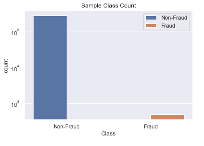
Businesses benefit from data recorded from electronic transactions to mitigate the chance of fraudulent activity. As an example we perform a case study using the Fraud Detection dataset from Kaggle (‘https://www.kaggle.com/mlg-ulb/creditcardfraud#creditcard.csv’) which includes credit card transactions as samples. The dataset has 31 columns. These include the time of the transaction, the amount, whether it was fraud or not, and many dimensionless columns of converted sensitive data. With this data we may compare how fraud transactions compare to non-fraud transactions in multiple ways. We will explore how the time the transaction takes place can effect when fraud takes place, the statistical distributions between fraud and non-fraud, and how the features of the dataset may be connected. These insights should allow us to build a model that detects whether a transaction can be flagged as fraudulent.

In the accompanying Jupyter Notebook, we share our analysis of this dataset. Using the Python Pandas, Seaborn, and Scikit-Learn libraries we are able to gain valuable insights into the dataset. Due to the low number of fraud samples we have an unbalanced classification problem. The fraud samples make up only 0.17% of our dataset. When looking at how much each charge was, the fraud charges tend to be less than a value of $1,000. The number of fraud samples also varies by time of day, as there are specific hours fraudulent charges spike in frequency. We found the dimensionless columns of the dataset to be uncorrelated, but a select few did correlate with the transactions amount. One of the more useful discoveries was found in comparing the empirical cumulative distribution for the fraud/non-fraud classes for each feature. Doing so revealed many of the features have visual differences in their statistical distributions between the two classes.

The rest of the analysis is a binary classification problem with uneven distributions. The two classes are fraud, or non-fraud. Since there is little information on the background of many of the columns, we choose not to normalize or preprocess the distributions of the features before fitting a model. In this example we will take an approach with a Random Forest Classifier. After parameter tuning using Grid Search and Cross Validation techniques, it was found that 160 trees in the forest with a maximum depth of 8 gave the best score. The analysis also searched over a select few oversampling parameters. The scoring method was done using Receiver Operator Characteristic Area Under Curve (ROC AUC). This method helps test the true detection and false positive rates, which is beneficial with uneven classes due to the lack of sensitivity in other binary classification scoring methods (i.e. accuracy or log-loss). Our final method had a successful ROC AUC scoring of 0.94, where the highest score is 1. It missed 12 fraud samples out of 102, and misclassified 27 non-fraud out of approximately 57,000. Finally, we tested feature importance by running experiments on our best model while removing a single feature at a time. In this way, we are able to see what features improve or decrease our ROC AUC scoring. Many of the features may be dropped, while the three most important features under this model are V14, V4, and Amount.

We were successful at building an analysis pipeline with a model that had strong ability at classifying fraud or non-fraud samples, using a Random Forest Classifier for our model. It attained an ROC AUC score of 0.94. Given more time or resources we would be able to further explore the feature set and parameter space of our forest using extensive grid searches. Other future directions would also include testing various resampling methods to improve the class balance.

NHL 2017-2018 Salary Analysis

https://github.com/willdupree90/NHL-2017-2018-Salary-Analysis/blob/master/NHL%202017-2018%20Salary%20Data%20Cleaning%20%26%20EDA.ipynb

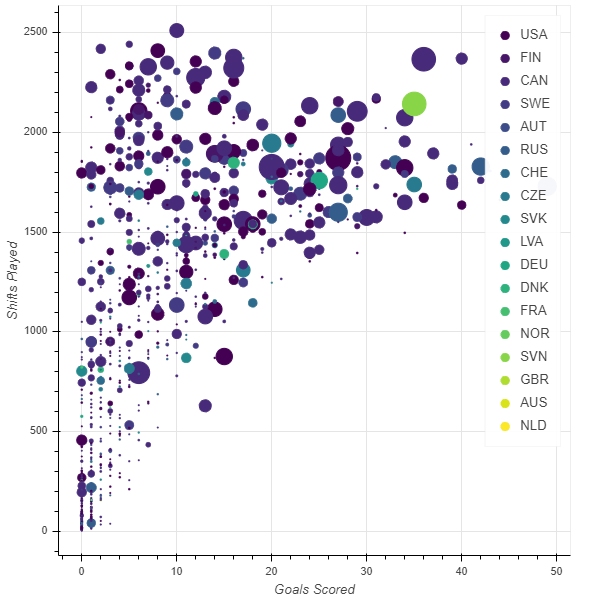
The NHL playoffs are just around the corner, so the perfect opportunity to combine our passion of data analytics and hockey into one project was formed. The Hockey Abstract, a website that shares a wide variety of player statistics shares seasonal data on their website. With over 200 different stats reported, it serves as a great data set to explore hockey and predictive capabilities on continuous variables. In this project we set out to predict a player’s salary based on the statistics found from the Hockey Abstract (http://www.hockeyabstract.com/testimonials/nhl2017-18).

We broke the bulk of the project into two Jupyter Notebooks. They are split between data cleaning and exploratory data analysis (EDA), and model building. The data comes from the 2017-2018 season, and contains fan sources as well as stats directly from the NHL. The raw file is an Excel Pivot Table. It has several different pages of statistics, as well as a Legend and About page. This analysis makes use of the first page of data, where the Legend is used for flattening the pivot table into a Pandas dataframe in Python. We explore the data, and eventually automate the processing into Pandas by creating our own abbreviations. On top of the importing process, some of the data also needed cleaning, as it was missing values in some of the columns. A background in hockey helps fill in missing values for players such as shoot out-shots, since if you don’t play in a shoot-out you simply have zero. While others required some thought such as missing draft information. We share our flattened and cleaned data in the files: nhl_2017_18_condensed.csv, nhl_2017_18_numeric_data.csv, and nhl_2017_18_text_data.csv.

Our analysis took advantage of the Python Bokeh library, performing the majority of the EDA by creating three interactive bar plots that a user can explore. These can be found in the 3 notebooks having Interactive Graph in their title. They create bar graphs comparing a variety of stats for 1 to 10 top players/teams, as well as scatter plots to visualize the salary and correlation of two recorded statistics. The interactive route made analysis easier, so as not to have to make many calls to Matplotlib to create all the required plots. Also, users who may not know as much Python can make quick use of the interactive functionality.

The second half of this project worked towards the main goal of predicting player salary from the given dataset. We made use of the numeric columns, as well as creating dummy variables from categorical text columns. After a first pass it became clear that Linear Regression, with no extra penalization, would be best. The Ridge method, which uses L2 normalization to keep model coefficients low, did not outperform Linear Regression. This was shown using parameter tuning of Ridge and comparing graphically to Linear Regression. Instead we used a forward wrapping method combined with k-fold cross validation to find the most influential features, and keep them for fitting a model. The model was successful with an R^2 score of 0.78 on the training data, and 0.75 on unseen test data. The most influential statistic was found to be Point Sharing, a catch all that follows how well a player contributes to the point’s standings of their team. It was closely followed by a given team’s expected goals based on when a player is on the ice.

Given more time we could improve our method with a more adhoc approach to explore what caused the model to predict a small number of unphysical salaries, shown by negative values. As we were using multidimensional regression that uses a hyperplane we could not quickly visualize an issue and track it down. Other avenues for future improvement would be including text based analysis on a player’s choice of equipment.